Semidefinite programming

From Wikipedia, the free encyclopedia

Jump to: navigation, search

Semidefinite programming (SDP) is a subfield of convex optimization concerned with the optimization of a linear objective function over the intersection of the cone of positive semidefinite matrices with an affine space, i.e., a spectrahedron.
Semidefinite programming is a relatively new field of optimization which is of growing interest for several reasons. Many practical problems in operations research and combinatorial optimization can be modeled or approximated as semidefinite programming problems. In automatic control theory, SDP's are used in the context of linear matrix inequalities. SDPs are in fact a special case of cone programming and can be efficiently solved by interior point methods. All linear programs can be expressed as SDPs, and via hierarchies of SDPs the solutions of polynomial optimization problems can be approximated. Finally, semidefinite programming has been used in the optimization of complex systems.

Motivation and definition

Initial motivation

A linear programming problem is one in which we wish to maximize or minimize a linear objective function of real variables over a polyhedron. In semidefinite programming, we instead use real-valued vectors and are allowed to take the dot product of vectors. Specifically, a general semidefinite programming problem can be defined as any mathematical programming problem of the form

$\begin{array}{rl} {\displaystyle \min_{x^1, \ldots, x^n \in \mathbb{R}^n}} & {\displaystyle \sum_{i,j \in [n]} c_{i,j} (x^i \cdot x^j)} \\ \text{subject to} & {\displaystyle \sum_{i,j \in [n]} a_{i,j,k} (x^i \cdot x^j) \leq b_k \qquad \forall k}. \\ \end{array}$

Equivalent formulations

An $n \times n$ matrix $M$ is said to be positive semidefinite if it is the gramian matrix of some vectors (ie. if there exist vectors $x^1, \ldots, x^n$ such that $m_{i,j}=x^i \cdot x^j$ for all $i,j$ ). If this is the case, we denote this as $M \succeq 0$ . Note that there are several other equivalent definitions of being positive semidefinite.
Denote by $\mathbb{S}^n$ the space of all real symmetric matrices. The space is equipped with the inner product (where ${\rm tr}$ denotes the trace) $\langle A,B\rangle_{\mathbb{S}^n} = {\rm tr}(A^T B) = \sum_{i=1,j=1}^n A_{ij}B_{ij}.$
We can rewrite the mathematical program given in the previous section equivalently as

$\begin{array}{rl} {\displaystyle\min_{X \in \mathbb{S}^n}} & \langle C, X \rangle_{\mathbb{S}^n} \\ \text{subject to} & \langle A_k, X \rangle_{\mathbb{S}^n} \leq b_k, \quad k = 1,\ldots,m \\ & X \succeq 0 \end{array}$

where entry $i,j$ in $C$ is given by $c_{i,j}$ from the previous section and $A_k$ is an $n \times n$ matrix having $i,j$ th entry $a_{i,j,k}$ from the previous section.
Note that if we add slack variables appropriately, this SDP can be converted to one of the form

$\begin{array}{rl} {\displaystyle\min_{X \in \mathbb{S}^n}} & \langle C, X \rangle_{\mathbb{S}^n} \\ \text{subject to} & \langle A_i, X \rangle_{\mathbb{S}^n} = b_i, \quad i = 1,\ldots,m \\ & X \succeq 0. \end{array}$

For convenience, an SDP may be specified in a slightly different, but equivalent form. For example, linear expressions involving nonnegative scalar variables may be added to the program specification. This remains an SDP because each variable can be incorporated into the matrix $X$ as a diagonal entry ( $X_{ii}$ for some $i$ ). To ensure that $X_{ii} \geq 0$ , constraints $X_{ij} = 0$ can be added for all $j \neq i$ . As another example, note that for any positive semidefinite matrix $X$ , there exists a set of vectors $\{ v_i \}$ such that the $i$ , $j$ entry of $X$ is $X_{ij} = (v_i, v_j)$ the scalar product of $v_i$ and $v_j$ . Therefore, SDPs are often formulated in terms of linear expressions on scalar products of vectors. Given the solution to the SDP in the standard form, the vectors $\{ v_i \}$ can be recovered in $O(n^3)$ time (e.g., by using an incomplete Cholesky decomposition of X).

Duality theory

Definitions

Analogously to linear programming, given a general SDP of the form

(the primal problem or P-SDP), we define the dual semidefinite program (D-SDP) as

$\begin{array}{rl} {\displaystyle\max_{y \in \mathbb{R}^m}} & \langle b, y \rangle_{\mathbb{R}^m} \\ \text{subject to} & {\displaystyle\sum_{i=1}^m} y_i A_i \preceq C \end{array}$

where for any two matrices $P$ and $Q$ , $P \succeq Q$ means $P-Q \succeq 0$ .

Weak duality

The weak duality theorem states that the value of the primal SDP is at least the value of the dual SDP. Therefore, any feasible solution to the dual SDP lower-bounds the primal SDP value, and conversely, any feasible solution to the primal SDP upper-bounds the dual SDP value. This is because

$\langle C, X \rangle - \langle b, y \rangle = \langle C, X \rangle - \sum_{i=1}^m y_i b_i = \langle C, X \rangle - \sum_{i=1}^m y_i \langle A_i, X \rangle = \langle C - \sum_{i=1}^m y_i A_i, X \rangle \geq 0,$

where the last inequality is because both matrices are positive semidefinite.

Strong duality

Under a condition known as Slater's condition, the value of the primal and dual SDPs are equal. This is known as strong duality. Unlike for linear programs, however, not every SDP satisfies strong duality; in general, the value of the dual SDP may lie strictly below the value of the primal.
(i) Suppose the primal problem (P-SDP) is bounded below and strictly feasible (i.e., there exists $X_0\in\mathbb{S}^n, X_0\succ 0$ such that $\langle A_i,X_0\rangle_{\mathbb{S}^n} = b_i$ , $i=1,\ldots,m$ ). Then there is an optimal solution $y^*$ to (D-SDP) and

$\langle C,X^*\rangle_{\mathbb{S}^n} = \langle b,y^*\rangle_{\R^m}.$

(ii) Suppose the dual problem (D-SDP) is bounded above and strictly feasible (i.e., $\sum_{i=1}^m (y_0)_i A_i \prec C$ for some $y_0\in\R^m$ ). Then there is an optimal solution $X^*$ to (P-SDP) and the equality from (i) holds.

Examples

Example 1

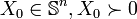
Consider three random variables $A$ , $B$ , and $C$ . By definition, their correlation coefficients 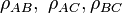$\rho_{AB}, \ \rho_{AC}, \rho_{BC}$ are valid if and only if

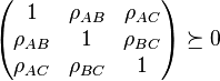
$\begin{pmatrix} 1 & \rho_{AB} & \rho_{AC} \\ \rho_{AB} & 1 & \rho_{BC} \\ \rho_{AC} & \rho_{BC} & 1 \end{pmatrix} \succeq 0$

Suppose that we know from some prior knowledge (empirical results of an experiment, for example) that $-0.2 \leq \rho_{AB} \leq -0.1$ and $0.4 \leq \rho_{BC} \leq 0.5$ . The problem of determining the smallest and largest values that $\rho_{AC} \$ can take is given by:

minimize/maximize $x_{13}$

subject to

$-0.2 \leq x_{12} \leq -0.1$

$0.4 \leq x_{23} \leq 0.5$

$x_{11} = x_{22} = x_{33} = 1 \$

$\begin{pmatrix} 1 & x_{12} & x_{13} \\ x_{12} & 1 & x_{23} \\ x_{13} & x_{23} & 1 \end{pmatrix} \succeq 0$

we set $\rho_{AB} = x_{12}, \ \rho_{AC} = x_{13}, \ \rho_{BC} = x_{23}$ to obtain the answer. This can be formulated by an SDP. We handle the inequality constraints by augmenting the variable matrix and introducing slack variables, for example
$\mathrm{tr}\left(\left(\begin{array}{cccccc} 0 & 1 & 0 & 0 & 0 & 0\\ 0 & 0 & 0 & 0 & 0 & 0\\ 0 & 0 & 0 & 0 & 0 & 0\\ 0 & 0 & 0 & 1 & 0 & 0\\ 0 & 0 & 0 & 0 & 0 & 0\\ 0 & 0 & 0 & 0 & 0 & 0\end{array}\right)\cdot\left(\begin{array}{cccccc} 1 & x_{12} & x_{13} & 0 & 0 & 0\\ x_{12} & 1 & x_{23} & 0 & 0 & 0\\ x_{13} & x_{23} & 1 & 0 & 0 & 0\\ 0 & 0 & 0 & s_{1} & 0 & 0\\ 0 & 0 & 0 & 0 & s_{2} & 0\\ 0 & 0 & 0 & 0 & 0 & s_{3}\end{array}\right)\right)=x_{12} + s_{1}=-0.1$
Solving this SDP gives the minimum and maximum values of $\rho_{AC} = x_{13} \$ as $-0.978$ and $0.872$ respectively.

Example 2

Consider the problem

minimize $\frac{(c^T x)^2}{d^Tx}$

subject to $Ax +b\geq 0$

where we assume that $d^Tx>0$ whenever $Ax+b\geq 0$ .
Introducing an auxiliary variable $t$ the problem can be reformulated:

minimize $t$

subject to $Ax+b\geq 0, \, \frac{(c^T x)^2}{d^Tx}\leq t$

In this formulation, the objective is a linear function of the variables $x,t$ .
The first restriction can be written as

$\textbf{diag}(Ax+b)\geq 0$

where the matrix $\textbf{diag}(Ax+b)$ is the square matrix with values in the diagonal equal to the elements of the vector $Ax+b$ .
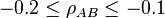
The second restriction can be written as

$td^Tx-(c^Tx)^2\geq 0$

or equivalently

det $\underbrace{\left[\begin{array}{cc}t&c^Tx\\c^Tx&d^Tx\end{array}\right]}_{D}\geq 0$

Thus $D \succeq 0$ .
The semidefinite program associated with this problem is

minimize $t$

subject to $\left[\begin{array}{ccc}\textbf{diag}(Ax+b)&0&0\\0&t&c^Tx\\0&c^Tx&d^Tx\end{array}\right] \succeq 0$

Example 3 (Goemans-Williamson MAX CUT approximation algorithm)

Semidefinite programs are important tools for developing approximation algorithms for NP-hard maximization problems. The first approximation algorithm based on an SDP is due to Goemans and Williamson (JACM, 1995). They studied the MAX CUT problem: Given a graph G = (V, E), output a partition of the vertices V so as to maximize the number of edges crossing from one side to the other. This problem can be expressed as an integer quadratic program:

Maximize $\sum_{(i,j) \in E} \frac{1-v_{i} v_{j}}{2},$ such that each $v_i\in\{1,-1\}$ .

Unless P = NP, we cannot solve this maximization problem efficiently. However, Goemans and Williamson observed a general three-step procedure for attacking this sort of problem:

Relax the integer quadratic program into an SDP.
Solve the SDP (to within an arbitrarily small additive error $\epsilon$ ).
Round the SDP solution to obtain an approximate solution to the original integer quadratic program.

For MAX CUT, the most natural relaxation is

$\max \sum_{(i,j) \in E} \frac{1-\langle v_{i}, v_{j}\rangle}{2},$ such that $\lVert v_i\rVert^2 = 1$ , where the maximization is over vectors $\{v_i\}$ instead of integer scalars.

This is an SDP because the objective function and constraints are all linear functions of vector inner products. Solving the SDP gives a set of unit vectors in $\mathbf{R^n}$ ; since the vectors are not required to be collinear, the value of this relaxed program can only be higher than the value of the original quadratic integer program. Finally, a rounding procedure is needed to obtain a partition. Goemans and Williamson simply choose a uniformly random hyperplane through the origin and divide the vertices according to which side of the hyperplane the corresponding vectors lie. Straightforward analysis shows that this procedure achieves an expected approximation ratio (performance guarantee) of 0.87856 - ε. (The expected value of the cut is the sum over edges of the probability that the edge is cut, which is proportional to the angle $\cos^{-1}\langle v_{i}, v_{j}\rangle$ between the vectors at the endpoints of the edge over $\pi$ . Comparing this probability to $(1-\langle v_{i}, v_{j}\rangle)/{2}$ , in expectation the ratio is always at least 0.87856.) Assuming the Unique Games Conjecture, it can be shown that this approximation ratio is essentially optimal.
Since the original paper of Goemans and Williamson, SDPs have been applied to develop numerous approximation algorithms. Recently, Prasad Raghavendra has developed a general framework for constraint satisfaction problems based on the Unique Games Conjecture.^[1]

Algorithms

There are several types of algorithms for solving SDPs. These algorithms output the value of the SDP up to an additive error $\epsilon$ in time that is polynomial in the program description size and $\log (1/\epsilon)$ .

Interior point methods

Most codes are based on interior point methods (CSDP, SeDuMi, SDPT3, DSDP, SDPA). Robust and efficient for general linear SDP problems. Restricted by the fact that the algorithms are second-order methods and need to store and factorize a large (and often dense) matrix.

Bundle method

The code ConicBundle formulates the SDP problem as a nonsmooth optimization problem and solves it by the Spectral Bundle method of nonsmooth optimization. This approach is very efficient for a special class of linear SDP problems.

Other

Algorithms based on augmented Lagrangian method (PENSDP) are similar in behavior to the interior point methods and can be specialized to some very large scale problems. Other algorithms use low-rank information and reformulation of the SDP as a nonlinear programming problem (SPDLR).

Software

The following codes are available for SDP:
SDPA, CSDP, SDPT3, SeDuMi, DSDP, PENSDP, SDPLR, ConicBundle
SeDuMi runs on MATLAB and uses the Self-Dual method for solving general convex optimization problems.

Applications

Semidefinite programming has been applied to find approximate solutions to combinatorial optimization problems, such as the solution of the max cut problem with an approximation ratio of 0.87856. SDPs are also used in geometry to determine tensegrity graphs, and arise in control theory as LMIs.

Ajay Shankar Bidyarthy, Systems Research Intern, TCS - TRDDC Pune

Monday, May 28, 2012